Molecular Dynamics: Non-bonded interactions

Molecular Mechanics (MM) is a powerful computational method that uses classical physics to simulate the behavior of molecules at the atomic level. By approximating a molecular system as a “balls and springs” model, where the atoms are represented as balls and the bonding interactions as springs, MM is able to predict the structure, properties, and dynamics of molecules with a high degree of accuracy.

Despite this simplification, constructing a realistic model of a molecule is not a trivial task and requires the calculation of its potential energy.

The potential energy of a molecule arises from the bonding interactions between atoms, and also from non-bonding interactions. Therefore, the potential energy of a molecular system at a given configuration $R$ can be expressed as:

$$E_{MM}(R) = E_{bond} + E_{non-bond}$$

You can find a detailed description of bonding terms in other articles. Here we will dive deeper on the different terms contributing to the non-bonding interactions.

Types of non-bonding interactions

When computing the energy of a molecular system we have to account for all the forces acting between non-bonding atoms. Such interactions can be mainly divided into two categories:

• Van der Waals ($E_{vdW}$)
• Electrostatic ($E_{el}$)

Both of them only consider the distance between two atoms and, therefore, can also be named pair interactions. Generally, we have non-bonded interactions in atoms that are not connected or connected by more than three bonds (1-5 connections and beyond). The overall equation for the non-bonded energy can be expressed as:

$$E_{non-bond}= E_{vdW} + E_{el}$$

While the explicit expression is more complex and it looks like this:

$$E_{non-bond}= \sum_{i=1} \sum_{j=i+1}\left(4\epsilon_{ij}\left[\left(\frac{\sigma_{ij}}{r_{ij}}\right)^{12}- \left(\frac{\sigma_{ij}}{r_{ij}}\right)^{6}\right] + \frac{q_iq_j}{4\pi\epsilon_0r_{ij}}\right)$$

The summatories are needed to account for all the possible pair interactions that, in a molecule composed of $N$ atoms are $\frac{N(N-1)}{2}$. As we can see, the entity of $E_{non-bond}$ largely depends on the distance between the examined pair of atoms.

While the computation of the bonding terms goes with $O(N)$, the non-bonded terms actually depend on the square of the number of atoms $O(N^2)$. This means that the number of non-bonded terms scales quadratically with the number of atoms in the system. Therefore, in large molecules (proteins, nucleic acids,…) the majority of the terms of a MM simulation are the non-bondings and becomes crucial to decide which ones to include in the potential energy equation.

Van der Waals interactions

The $E_{vdW}$ contribution is needed to describe the Van der Waals attractions and repulsions in atoms that are not directly bonded. The value of the energy is the result of a balance between attractive and repulsive forces. Therefore, it mostly depends on the interatomic distance, as they modulate the intensity of the attractions and repulsions between atoms.

Naturally, for large atomic distances the interactions are non-existent and the $E_{vdW}$ value is zero. Conversely, when atoms are very close the repulsion becomes stronger. Among these two situations, we have a set of intermediate circumstances where the atoms are not too close or too far and there is a slight attraction due to induced dipole-dipole interactions.

Globally, $E_{vdW}$ has to be positive at small distances, slightly negative at intermediate distances, and slowly approach zero when the atoms are split (green line in Figure 1).

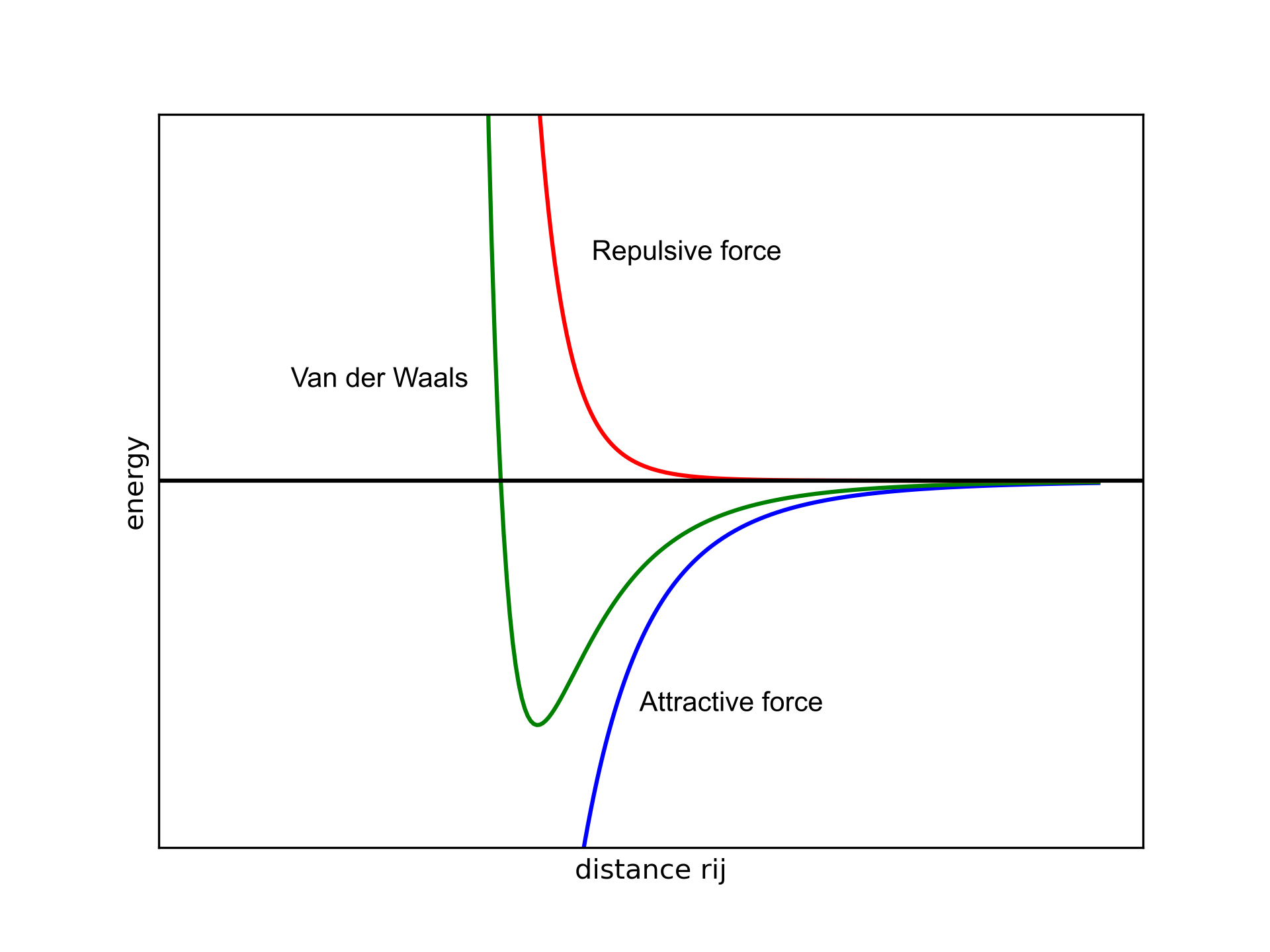
Figure 1. Van der Waals potential as a function of the distance between two atoms $i$ and $j$.

This interaction can be fitted by various functions, one of the most common is the Lennard-Jones (LJ) potential:

$$E_{vdW}= \sum_{i=1} \sum_{j=i+1}4\epsilon_{ij}\left[\left(\frac{\sigma_{ij}}{r_{ij}}\right)^{12}- \left(\frac{\sigma_{ij}}{r_{ij}}\right)^{6}\right]$$

The attractive part (blue line) has a $\sigma^6$ dependence, while the repulsive (red line) part shows a $\sigma^{12}$ dependence. The distance between atoms ($r_{ij}$) is in the denominator and the high exponentials are needed to make sure that $E_{vdW}$ rapidly goes to zero when $r_{ij}$ increases. This allows us to decide on a distance threshold so that if two atoms are separated by more than a given radius we can avoid computing those terms since the contribution would be negligible.

For instance, when parametrizing a Force field we may decide to cut-off distances at 10 A° and ignore the Van der Waals interactions arising from two atoms separated by more than 10 $\mathring A$.

Other functions can be used to model Van der Waals interactions, such as the Buckingham and the Morse potential.

These two potentials differ from the previous one for mainly two reasons.

• The mathematical form used to describe the repulsive force, involves exponential functions that are slower to determine with respect to simple operations such as additions or multiplications.

• The number of parameters contained, LJ has two parameters while the others have three. This makes the LJ potential faster to compute but, at the same time, less accurate with respect to the other two potentials. Also, in this case, the Morse potential provides the most accurate description among the available methods.

Electrostatic interactions

The other contribution to the non-bonded energy is due to the fluctuation of the electronic cloud generating positively and negatively charged regions. To model the effect of this process we need to add an electrostatic term ($E_{el}$).

The lowest level of approximation to model the electrostatic interaction between two atoms is to consider them as point charges, and represent $E_{el}$ by the Coulomb potential:

$$E_{el}= \sum_i\sum_{j=i+1} \frac{q_iq_j}{4\pi\epsilon_0r_{ij}}$$

where the two parameters $q_i$ and $q_j$ are the charges of the $i$-th and $j$-th atoms, and the distance $r_{ij}$ is the variable.

The polarization may arise from atoms belonging to the same molecule (intramolecular) or to different molecules (intermolecular). The electrostatic potential is not easy to compute because $r_{ij}$ has no exponential and the function goes to zero more smoothly than the $E_{vdW}$.

In other words, the interactions between atoms are present even at high distances. So we can’t cut off the interactions over a certain radius as we previously saw for Van der Waals. The electrostatic terms are therefore the rate-limiting step in a MM simulation because of the huge number of terms to compute ($O(N^2)$).