How to compute the RMSF using GROMACS

GROMACS is one of the most widely used software for conducting molecular simulations. On this website, you will find different GROMACS tutorials that will help you to run protein simulations.

However, once your simulation is complete, you should also be interested to continue with the analysis of the resulting trajectory. Among different analyses at your disposal, one that often holds great importance is the Root Mean Square Fluctuation, fondly known as RMSF. In this article, you’ll learn about the concept of RMSF and gain practical insights into computing it using GROMACS’ dedicated gmx rmsf module.

What is the RMSF?

The Root Mean Square Fluctuation (RMSF) is an important structural feature that one can study in Molecular Dynamics (MD). It measures the fluctuation of an atom or a group of atoms (e.g., a protein residue) along the course of a simulation, and is useful to identify the most mobile regions of our system providing valuable insights on the structural dynamics of the system.

The RMSF ($\rho$) is computed as the square root of the variance of the fluctuation around the average position. In other words, we compute the root mean square of the deviations of the atomic positions from their mean positions over a series of time steps of a molecular dynamics simulation.

For a generic atom $i$ we have that:

$$ \rho_i = \sqrt {\big \langle ( r_i - \langle r_i \rangle)^2 \big \rangle } $$

where $r_i$ represent the coordinates of atom $i$, and $\langle r_i \rangle$ its ensemble average position.

The interpretation of the RMSF value is quite straightforward:

• A region characterized by high RMSF values indicates high divergence from the average position and therefore high structural mobility.

• The opposite is true for regions displaying low RMSF values which will not deviate much from the average position, meaning that they are more rigid during the simulation.

RMSD vs RMSF

You may notice that the basic concept of this feature is somewhat similar to the concept of Root Mean Square Deviation (RMSD). However, the information that we retrieve from the two analyses is different.

• The RMSD shows how much the molecule of interest deviates from its initial structure over the course of the simulation. Therefore, it is used as an indicator of convergence and is generally plotted as a function of time. When the RMSD curve becomes flat the system is not changing significantly anymore and it can be considered equilibrated.

• The RMSF determines the fluctuation of an atom (or a group of atoms) during the simulation. This means that it is generally used to check the flexibility of residues within a protein during the course of the simulation. For this reason, it needs to be plotted against the residue number to measure the contributions of different amino acids to the overall molecular motion.

Typically, one would perform an RMSD analysis to verify that the value reached a plateau and that the structure has equilibrated.

Subsequently, you may want to perform the analysis of the RMSF during the equilibrated portion of the trajectory to observe which residues fluctuate the most even when the structure is stable.

The gmx rmsf command

You can use this tool to compute the RMSF of different residues during an MD simulation.

1

gmx rmsf -f simulation.xtc -s simulation.tpr -o rmsf.xvg -res (-b 1000 -e 10000)

In protein simulation, we generally compute the RMSF of the $C_{\alpha}$ which gives us the fluctuation of the backbone for each residue. At the prompt, select the group C-alpha.

The RMSF will be computed from the average structure in the analyzed time frame and you will find the output in the rmsf.xvg file.

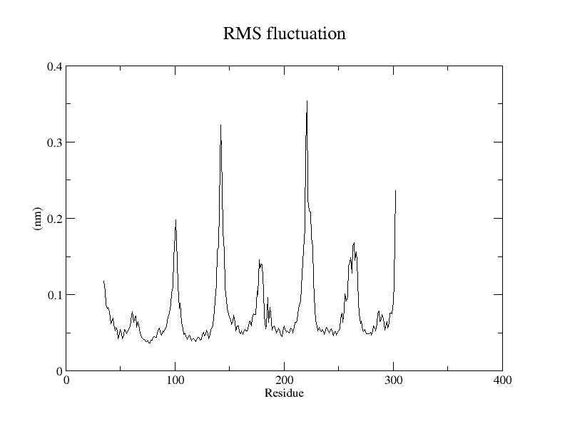
As usual, you can plot the resulting xvg file with your favorite tool. Here I showed you how you can plot it with Grace or Python.

Grace

1

xmgrace rmsf.xvg

Python

 1
 2
 3
 4
 5
 6
 7
 8
 9
10
11
12
13
14
15
16
17
18
19
20
21
22
23
24
25
26

# Importing the necessary libraries for plotting
import matplotlib.pyplot as plt
import numpy as np

# Loading data from the rmsf.xvg file, ignoring lines starting with "@" or "#"
res,rmsf = np.loadtxt("rmsf.xvg", comments=["@", "#"], unpack=True)

# Creating a figure and axis objects for the plot
fig = plt.figure(figsize=(10,5))
ax = fig.add_subplot(111)

# Filling the area between the x-values (res) and y-values (rmsf) with a semi-transparent black color
ax.fill_between(res,rmsf, color="black", linestyle="-", alpha=0.3)

# Plotting the line representing the RMSF values
ax.plot(res,rmsf, color="black", linestyle="-")

# Setting labels for the x-axis (residue) and y-axis (RMSF value)
ax.set_xlabel("residue")
ax.set_ylabel(r"C$_\alpha$ RMSF (nm)")

# Saving the plot as a PNG image with higher resolution (300 dpi)
plt.savefig("rmsf.png", format="png", dpi=300)

# Displaying the plot
plt.show()

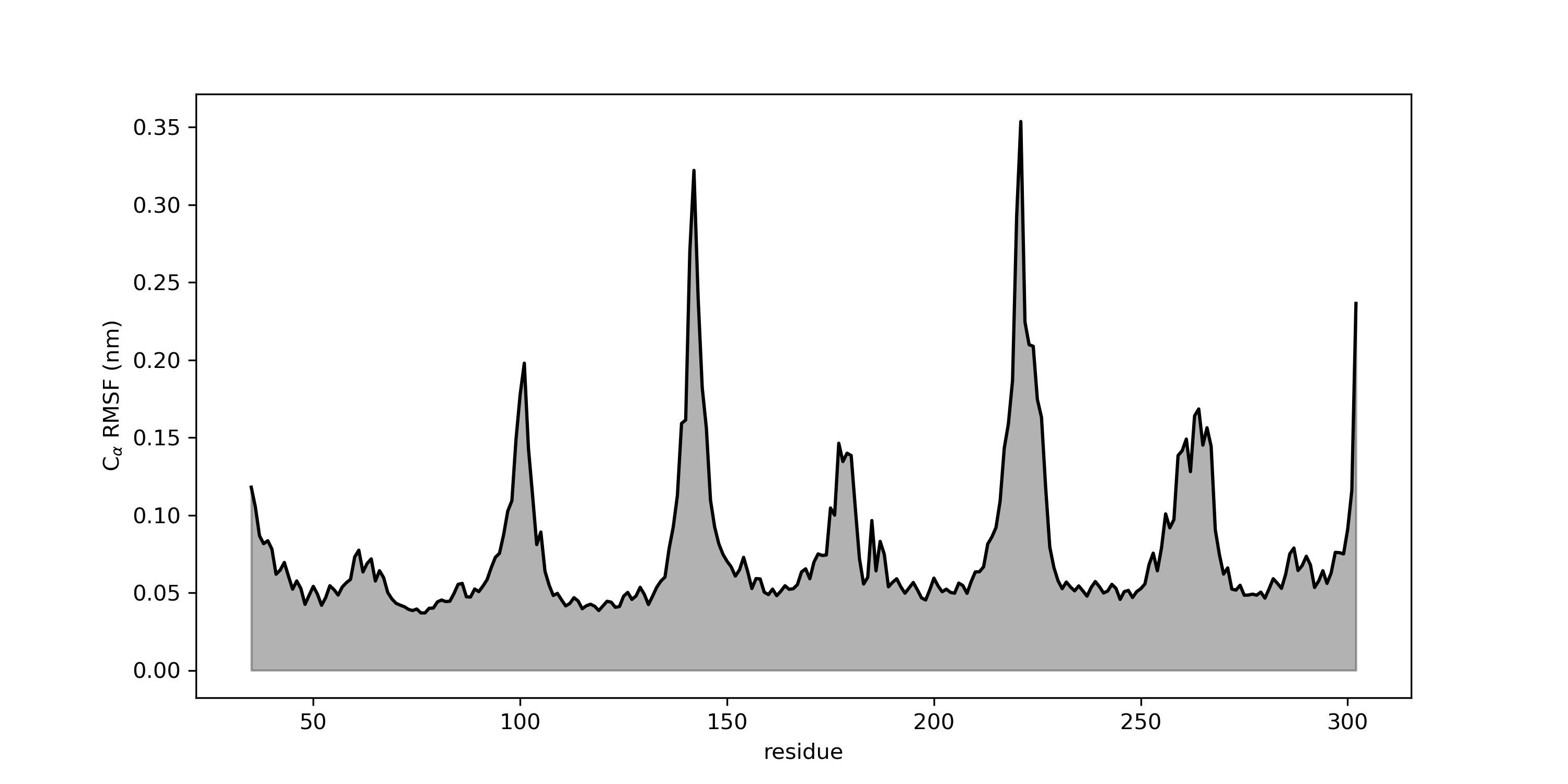
The spikes in RMSF correspond to the residues having wider fluctuation along the trajectory.

B-factor analysis with GROMACS

You can also use the gmx rmsf command to perform the B-factor analysis.

In this analysis, the RMSF values are converted into B-factors, offering a valuable measure of atom fluctuation within your system. These B-factor values are then efficiently writtein to a new PDB file, where they are conveniently placed in the last column (for an in-depth look at PDB formatting).

The usefulness of this approach becomes apparent when you utilize tools like PyMOL to import the PDB file and apply color schemes based on B-factor values to your molecular structure. This dynamic visualization offers a direct means of evaluating atom fluctuations within your molecular system.

To perform this analysis you will need to add the -oq flag to the previous command and decide how to name the output file (bfac.pdb).

1

gmx rmsf -f simulation.xtc -s simulation.tpr -o rmsf.xvg -oq bfac.pdb

The outcome is a PDB file enriched with B-factor data, ready for import into visualization tools like PyMOL or VMD. This file allows you to visually identify the most dynamic regions within your system, offering valuable insights into molecular mobility.