An Introduction to Enhanced Sampling and Metadynamics

If you’ve been following my blog, you’re probably familiar with my articles on the basics of Molecular Dynamics (MD) and using GROMACS for simulations.

While plain MD can be quite powerful, the harsh truth is that it often falls short for many complex problems. In this article, I’ll explain why enhanced sampling techniques are necessary in molecular simulations and introduce you to one of the most renowned methods: Metadynamics.

I will just give you an intuition of the method while I will save a more rigorous description of the method for a future post.

Challenges in Molecular Simulation

Since its inception, molecular simulation has been confronted with two primary challenges:

1. Model Accuracy: Creating a model that faithfully represents the real system of interest is crucial. Although this issue is critical, we will leave this to discuss another time ;)

2. Time-Scale Problem: Many processes in molecular simulation occur on timescales that are inaccessible to standard simulations. This limitation is known as the Time-Scale Problem or the Sampling Problem.

The second challenge is more tricky and is the primary driver for developing enhanced sampling methods. Let’s analyze it in more depth.

Rare Events and Enhanced Sampling

Imagine you want to simulate a process from state A to state B (e.g., DNA/protein folding, liquid-to-solid transition, ligand binding to a protein, …).

If the energy barrier between these two states is too high, starting your simulation in one state will likely trap you there for an extended period, restricting you to only one relevant state.

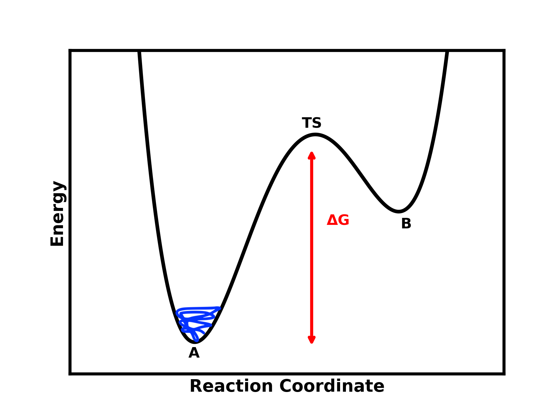
Figure 1: A two-step process where the simulation starts at state A and is unable to cross the energy barrier (ΔG) due to its height.

Turns out that high barriers separating different metastable states are very common in many natural phenomena. We call these phenomena “rare events”, characterized by long-lived metastable states separated by kinetic bottlenecks.

The situation gets even more complicated when considering a real free energy surface. It often resembles a rugged landscape with numerous peaks and valleys, each representing different states and transition barriers.

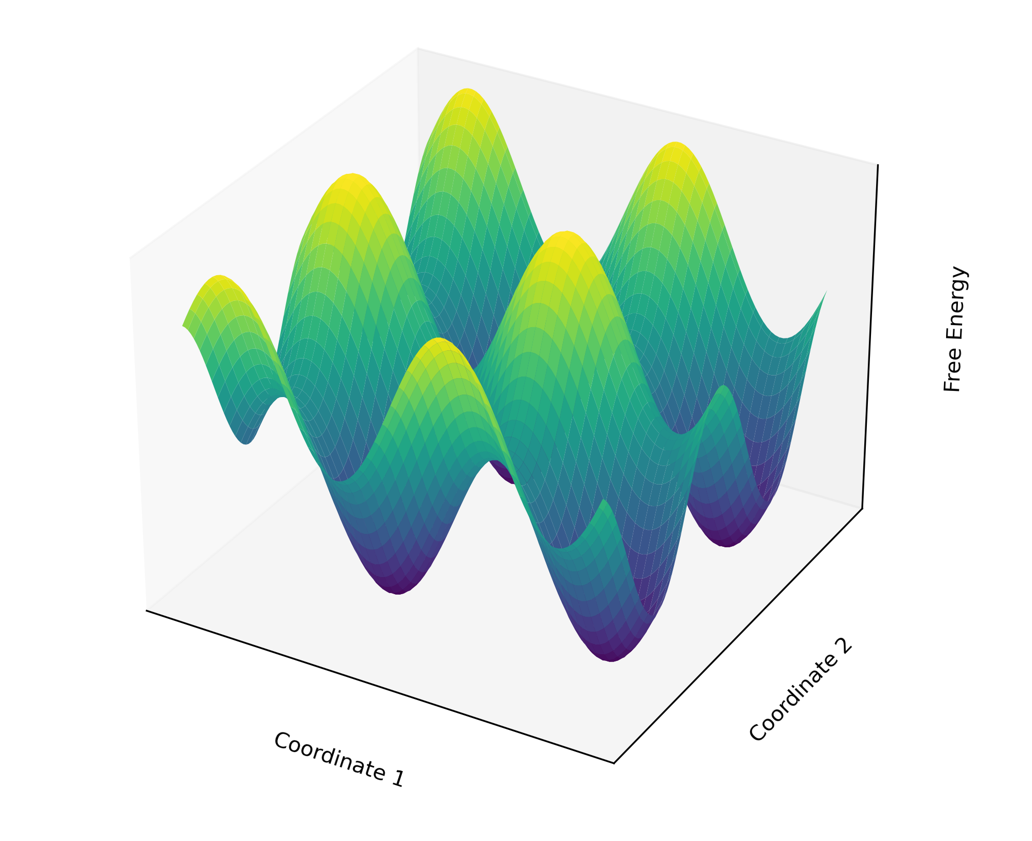
Figure 2: A rugged 3D free energy surface illustrating the complex landscape of multiple peaks and valleys.

In many practical cases, you might need to simulate your system for an impractically long time to visit all the relevant states. However, available computational resources typically only allow simulations on the nanosecond (ns) to microsecond (µs) timescale.

Hence, an unfeasible amount of simulation time is required.

This is why we need more efficient sampling techniques, known as Enhanced Sampling Methods, to “cross the barrier” and explore all the possible relevant conformations of the system. These methods help us overcome the limitations of traditional simulations by accelerating transitions between different metastable states.

Various methods have been developed to enhance sampling in molecular simulations, such as umbrella sampling, metadynamics, steered molecular dynamics, adaptive biasing force, replica exchange, and parallel tempering,…

The list goes on, but in this discussion, we will focus specifically on Metadynamics.

Metadynamics

One effective approach to accelerate rare events in molecular simulations is Metadynamics.

Although the mathematics behind Metadynamics can be complex, the core concept is intuitive and easy to visualize. This makes it accessible even for those without a strong mathematical background.

Conceptual Overview

Consider again the scenario where you need to cross an energy barrier.

One way to achieve this is by placing a bias potential, which essentially “fills” the well of the first minimum (state A), allowing you to cross the barrier and reach state B.

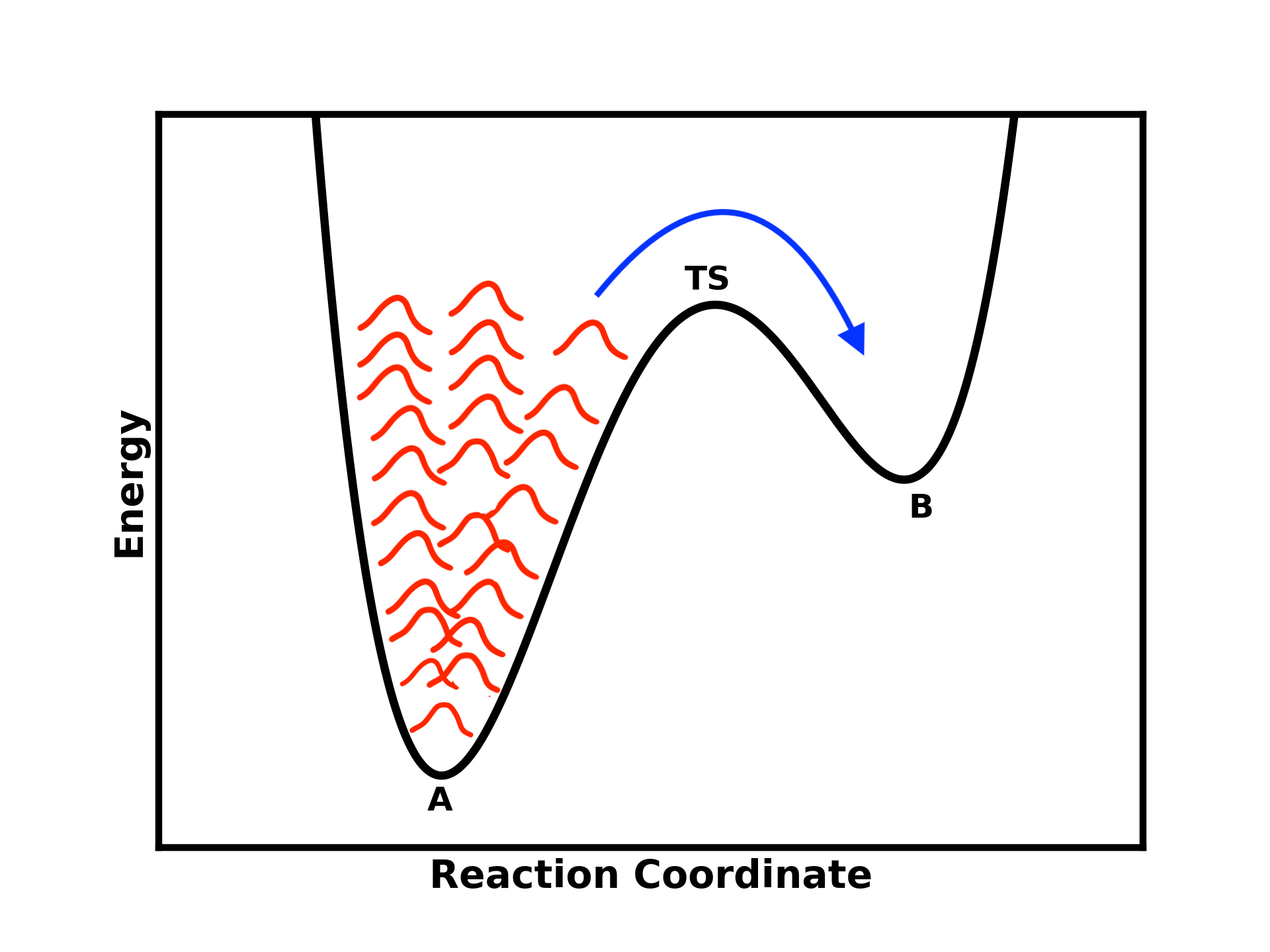
Figure 3: Illustration of Metadynamics adding a Gaussian-shaped bias potential to help the system escape the free energy minima and transition to other states

This is precisely what Metadynamics does. It adds a Gaussian-shaped bias potential to help escape the free energy minima and visit other states.

The idea is that you are depositing these Gaussian potentials in a history-dependent manner (keeping track of them), creating a repulsive potential that discourages the system from revisiting the same state and pushes it toward other states.

Once the well of state B is filled as well, the system is expected to move back to state A. Eventually, you will reach an almost flat energy landscape where the system can easily visit both states.

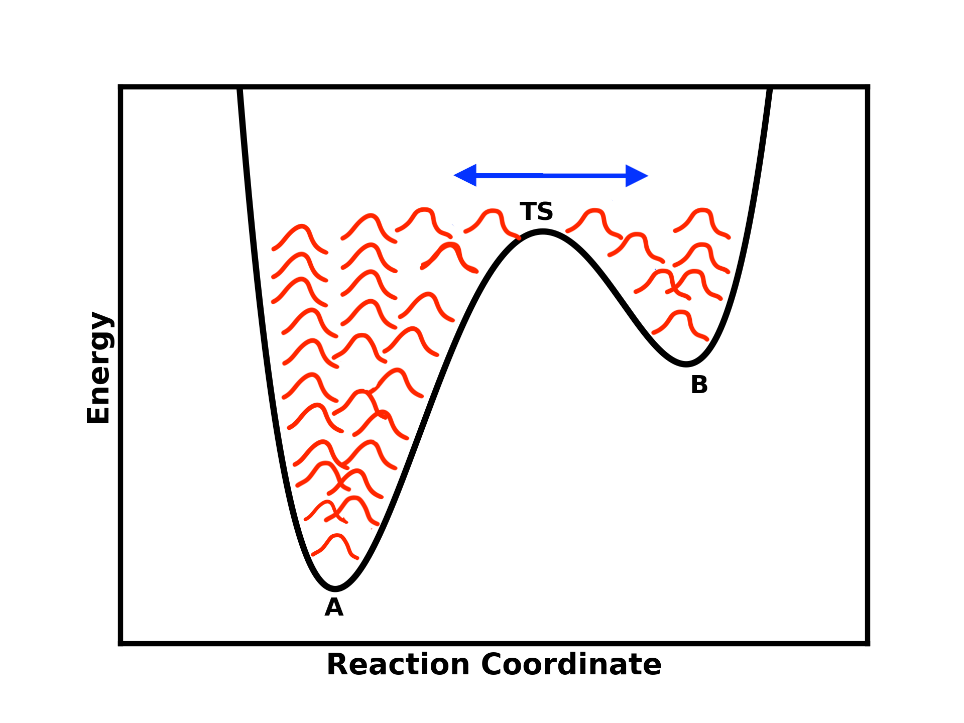
Figure 4: As more Gaussian potentials are added, the energy landscape flattens, allowing the system to transition more easily between states A and B.

Practical Implementation

Everything sounds great in theory, but you might be wondering: How do we achieve this in practice? What parameters do we need to choose to successfully implement Metadynamics?

Here’s a more structured approach to its practical implementation, which can be divided into three main steps.

Step 1: Collective Variables (CVs)

So previously we mentioned the fact that we need to add bias potential to accelerate transitions.

We don’t always know the right axis on which to project the free energy profile. In other words, we don’t know in advance the x-axis in the previous figure, and therefore, we don’t know the right coordinate we want to bias.

And here is where the tricky part comes in.

In order to perform a successful metadynamics run we first need to define a so-called Collective Variable (CV). You might have heard this already. A CV is a geometrical descriptor (a function of the coordinates of the system) that needs to be able to describe the process we want to study.

In other words, CVs should be able to (1) distinguish between different states and (2) represent the slow degrees of freedom in the process of interest.

It is only after a thoughtful selection of CVs that we can proceed to introduce bias into the system. If the CVs are poorly selected then we will see no transitions at all.

Selecting good CVs often requires a deep understanding of the system and the process of interest. It may involve trial and error and can benefit from prior knowledge or experimental data. This is the most difficult and also the most important parameter to choose and is almost always the bottleneck to a metadynamics experiment.

I will probably discuss this more in-depth in another article.

Step 2: Add Bias Potential

So the first step of a metadynamics run is to define a set of Collective Variables.

Once we have done that, as a second step we can start adding a biasing potential. This is constructed adaptively by depositing Gaussian-shaped potentials centered on the points visited by the CV during the simulation. Given that the CVs we choose are good enough, This allows the simulation to overcome free energy minima that would impede the observation of rare events in a reasonable time frame.

We need to define three key parameters related to the Gaussian potentials:

1. Deposition frequency: This parameter determines how frequently a Gaussian potential is placed. In other words, it controls the speed at which you are modifying the history-dependent bias. A higher frequency will lead to faster exploration but may result in a less accurate free energy estimate.

2. Gaussian width: This parameter sets the width of the Gaussian potentials being placed. A wider Gaussian will lead to a smoother free energy landscape but may miss fine details. Conversely, a narrower Gaussian can capture more detail but may lead to slower convergence.

3. Gaussian height: This parameter determines the height of the Gaussian potentials. A larger height will lead to faster exploration but may result in a less accurate free energy estimate.

Step 3: Estimate of Thermodynamics properties via Metadynamics

One immediate advantage of Metadynamics is that it can accelerate transitions between states.

However, the aspect that makes this method particularly popular is that from the bias potential, one can directly estimate the free energy surface (FES) as a function of the selected CVs without a priori knowledge of the energy landscape. The FES can be estimated directly from the bias potential by summing up the deposited Gaussians.

The key insight here is that by tracking all the Gaussians deposited during the run, the bias potential converges to the negative free energy plus a constant in the long-term limit. Go back to the earlier figures to see how the deposited Gaussians shape the free energy profile.

Furthermore, it is possible to obtain the FES, both for the biased CVs and for any other set of CVs, via reweighting.

Under certain conditions, one can also rescale simulation time to obtain rare-event kinetics from biased Metadynamics simulations.

What this means is that Metadynamics not only helps in crossing free energy barriers but also allows for the retrieval of thermodynamic properties, such as free energy. But it can also be used to retrieve kinetic rates of processes.

Well-Tempered Metadynamics

In standard metadynamics, Gaussian kernels of constant height are added for the entire course of a simulation. One disadvantage with this approach is that the system is prone to overfilling. This means that we will keep on adding more and more bias and eventually we might end up in regions with very high energy that we are not necessarily interested in exploring.

Additionally, with complex systems, standard metadynamics often struggle to converge; the free energy estimate oscillates around the true value without settling, making it difficult to determine when to stop the simulation.

For this reason, nowadays another method is more popular, especially for dealing with complex systems, namely Well-Tempered Metadynamics.

Here, we set an initial height of the Gaussian and then we decrease it with simulation time. So as the simulation progresses the bias also decreases leading to a smoother convergence. We obtain an estimate of the FES that converges to the exact result in the long time limit.

Furthermore, we have an additional parameter that we can use to tune the extent of the exploration of the free energy surface. This approach offers the possibility of controlling the regions of FES that are physically meaningful to explore.

By addressing overfilling and convergence issues, well-tempered metadynamics leaves us with just one remaining challenge: the choice of the CV.

PLUMED

Which software can you use to perform enhanced sampling?

The most popular software is PLUMED, an open-source, community-developed library that provides a wide range of different methods, which include:

• enhanced-sampling algorithms
• free-energy methods
• tools to analyze data produced by MD simulations.

PLUMED works together with some of the most popular MD engines, such as, such as GROMACS, Amber, OpenMM, and many more. and can also be used to enhance analysis tools like VMD. 

I plan to write articles on how to use PLUMED. In the meantime if you are interested you can read the documentation or explore examples from other users in the PLUMED-NEST repository.

Useful Readings

Some readings you may find useful:

• A review on enhanced sampling methods
• The original metadynamics paper
• The Well-Tempered Metadynamics paper
• A technical review on metadynamics
• If you prefer videos, I highly recommend this guide on YouTube